Posts

Showing posts with the label Analysis

GIS 6005 - Proportional Symbol and Bivariate Choropleth Mapping
Image
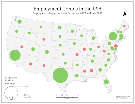
 While there are many ways to display data on a map, proportional symbol and bivariate choropleth mapping can be considered two methods that are technically challenging but significantly beneficial when executed correctly. The challenges proportional symbol maps can introduce include, but is not limited to, overlapping symbols, symbols that do not have enough variation in size, and accurately displaying positive and negative values. One of the maps created for this week's lab, as seen below, is an example of a proportional symbol map that has both positive and negative values. To properly display both sets of values, the GIS professional has to create additional attribute fields that separate the positive and negative values, followed by making the negative values positive. Once this is done. The data can be symbolized and displayed effectively.  Alternatively, bivariate choropleth mapping involves showing the relationship between two data variables. This is particularly benef...

GIS 6005 - Analytical Data

Image
When we think about using GIS to communicate information it can often be done with a single map. However, we often require additional 'help' relaying that information. This help can be in the form statistics and various graphs, which are derived from analysis of raw data. When the supplemental statistics and graphs are, then, combined with a map or multiple maps we create an infographic. The task for students this week was to create our own infographic that includes two maps, multiple charts and statistics stated in text format. The infographic I created highlights the relationship between smoking and reports of fair or poor health.  To create this infographic, data from County Health Rankings was combined with existing county GIS data to create two choropleth maps. The first map displays the percentage of adult smokers by county and the second map shows the percentage of adults that reported their health to be fair or poor. The maps are accompanied by two pie charts, a scatter...

GIS 5935 - Scale Effect and Spatial Data Aggregation

Image
As seen in the title, this week's module and lab covered two topics. The first topic was scale effect. In a world where we have various interactive maps at the palm of our hand, scale effect may not have the most blatantly obvious issue with viewing data. However, scale effect can have a wide-ranging impact on data we are using and collecting. Vector data, for example, created from imagery or raster data is only as good as the finest detail that can be seen. This means at a small scale the resolution is considered low and small features and intricacies are not visible. Larger features are the only items detectable or discernable. As such, fewer vertices and segments are used to represent a feature, which can lead to less accurate calculations that tend to have a smaller numerical account of the feature. The opposite is true for large scales.  The second topic covered this week was spatial data aggregation. This refers to the combining of data into a boundary, which in turn gen...

GIS 5935 - Surfaces - TINs and DEMs

Image
Having moved on from the modules regarding data quality, this week we were introduced to surfaces and surface models, more specifically Triangulated Irregular Networks (TINs) and Demographic Elevation Models (DEMs). TINs are based on vector data and are made up of a series of linked triangles that vary in shape and size, but display a 3D representation of a surface. DEMs are based on raster data, more specifically the spot heights associated with each grid part of a raster.  For this lab we were tasked with creating a TIN and DEM, as well as displaying contours based on both of them. We were then tasked with comparing the contours produced by both. Below I have included images of my results.  (a) Contour lines based on the TIN (b) Contour lines based on the DEM The contours produced as a result of the TIN appear to be more jagged, while the contours produced from the DEM have a smoother appearance. There is also a noticeable difference between the derived contours in areas...

GIS 5935 - Data Quality Assessment

Image
Like the second assignment, this module continues to focus on data quality. More specifically, this week focused on data quality of road networks. As such, we were tasked with performing a comparative assessment to determine the completeness of a street centerline shapefile and a Topologically Integrated Geographic Encoding and Referencing (TIGER) road shapefile for Jackson County, Oregon.  To perform this assessment we utilized a non standard method, based on that used by M. Haklay in the "Comparative Study of OpenStreetMap and Ordinance Survey datasets" in 2010. This included using a grid, which encompasses the study area, to clip the road network into smaller sections. These smaller sections give more detailed insight into areas which may be considered complete or incomplete. Once the roads were clipped to each grid cell/section the lengths were calculated and then compared.  My analysis determined that 134 of the grid cells/sections contained parts of the street cente...

GIS 5935 - Data Quality Standards

Image
Continuing on from the first week of GIS5935, this week we were introduced to the more common data quality standards used for cartographic and digital geospatial data. These standards were put in place by organizations, such as the United States Geological Survey (USGS) and the Federal Geographic Data Committee (FGDC), to "provide a common language for reporting accuracy to facilitate the identification of spatial data for geographic applications" (FGDC, 1998). In particular, the lab allowed us to perform our own positional accuracy tests using the National Standard for Spatial Data Accuracy (NSSDA) standards.  The NSSDA standard follows a seven step process which includes the following:      1. Determining if the test should be for horizontal accuracy, vertical accuracy or both.      2. Selecting test points from the data set being evaluated      3. Selecting an independent data set of higher accuracy that corresponds to the data s...

GIS 5100 - Least-Cost Analysis

Image
 This is my second blog post for Module 6 and the focus is Least-Cost analysis. We were tasked with performing an analysis and producing a map that models a corridor that black bears would use to travel between two protected areas in Coronado National Forest. To do this we had to take into consideration criteria that suits black bear habitats. As such the following is the criteria: Criteria 1: Landcover best suited for black bear habitats, such as forested areas. Criteria 2: Distance from roadways. The farther the better. Criteria 3: Mid elevations. Ideally, 1200 to 2000 meters.  My process included the following steps. To model the corridor that black bears would use to travel between the two protected areas in Coronado National Forest I first created a ranked raster for elevation and landcover using the reclassify tool, followed by performing a Euclidean distance on the roads and reclassification to rank them as well. The ranked rasters were then combined using the Weighted ...

GIS 5100 - Suitability Analysis

Image
 Module 6 is here! For the 6th and final module students have been tasked with creating two blog posts. This is my first blog post for this module and the focus is Suitability Analysis. We were tasked with creating a suitability map which models and rates the best locations for development. To do this we had to take into consideration criteria that best determines suitable locations for development. As such, the following are the criteria: Criteria 1: Landcover best suited for development, such as agricultural or meadows. Criteria 2: Soil best suited for development. Criteria 3: Gentle slopes . Criteria 4: Areas more than 1000 ft away from streams. Criteria 5: Areas that are near to roads.  For each of the above criteria rasters were ranked or created then ranked via reclassification. This step was followed by performing a weighted overlay analysis, which combined the criteria at various weights to determine the most suitable areas for development. The weighted analysis was pe...

GIS 5100 - Damage Assessment

Image
 As a follow up to the last module on Coastal Flooding, this module focuses on the damage assessment after a coastal flooding event, such as a hurricane and it's associated storm surge. In 2012 hurricane Sandy impacted the north eastern coast of the US and left behind monumental damage. This week's module tasked students with performing their own analysis of a portion of the area impacted by hurricane Sandy. In the first instance we were required to create a map of hurricane Sandy's track. The following is my result:  We were then asked to mosaic imagery of the New Jersey shoreline pre hurricane Sandy and post hurricane Sandy, followed by doing a comparative desktop study to assess the damage caused by the storm. To assess the damage a point was created for each building in the study area and the structure damage, wind damage and inundation was determined and ranked based on FEMA standards. The following is an image of the building points based on structural damage:  To f...

GIS 5100 - Coastal Flooding

Image
During this week's module, module 4, we learned about Coastal Flooding, which can take place at various speeds, including rapidly via surge or slowly via sea level rise. This week we were tasked with performing analysis on the New Jersey shoreline and the coast of Collier County in Florida. In New Jersey we used LiDAR data to evaluate change post hurricane Sandy. This analysis included observing the raw LiDAR data, followed by the creation of Digital Elevation Models (DEMs) of pre and post hurricane Sandy for comparison. A more recent building vector file was also used to assist in the assessment of change, although using more recent data should be used with caution as it does not always accurately depict change as a result of a disaster event. This is particularly true as more time passes. The following map displays elevation change on the New Jersey Shoreline.  Map depicting elevation change post hurricane Sandy.   For Collier County, Florida, we were tasked with determ...

GIS 5100 - Visibility Analysis

Image
For module 3 we continued learning about LiDAR data and analysis with the introduction of visibility analysis. The visibility analysis introduced included Line of Sight (LOS) analysis and View Shed analysis. The lab assignment supplemented the lectures by requiring the completion of four exercises. The following are the exercises and a bit of information about each:  Exercise 1: Introduction to 3D Visualization As the title suggests, this exercise introduced students to 3D visualizations. It began highlighting how 3D can be used and quickly moved into providing hands on experience in displaying and navigating 3D data in ArcGIS Pro, displaying 2D layers as 3D by extruding the 2D feature, and applying effects to the 3D data such as various types of illumination.  Exercise 2: Performing Line of Sight Analysis According to ESRI, line of sight analysis determines if two points in space are intervisible. Intervisibility can be impacted by and obstruction, such as a building, which i...

GIS 5100 - Forestry and LiDAR

Image
The second module of the Applications in GIS course introduced students to Watersheds and LiDAR. While I have previously been exposed to LiDAR, I had not had the opportunity to work with LiDAR data and manipulate it until this module. As such, it was exciting to be able to get this opportunity to learn about it. This week's lecture focused more on watershed analysis, while the lab focused on using LiDAR. The lab tasked students with creating a Digital Elevation Model (DEM) and Digital Surface Model (DSM), calculating forest height and calculating biomass. Below are maps that were produced as a result of the lab assignment.  Map of Canopy Density in the Big Meadows Area of Shenandoah National Park Map of Tree Heights in the Big Meadows Area of Shenandoah National Park LiDAR Scene and LiDAR Derived DEM in the Big Meadows Area of Shenandoah National Park While I enjoyed working with LiDAR data, exploring data in 3D and learning of its power in analysis, this type of data requires hard...