Posts

Showing posts with the label GIS

GIS 6005 - Proportional Symbol and Bivariate Choropleth Mapping
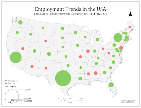
Image
 While there are many ways to display data on a map, proportional symbol and bivariate choropleth mapping can be considered two methods that are technically challenging but significantly beneficial when executed correctly. The challenges proportional symbol maps can introduce include, but is not limited to, overlapping symbols, symbols that do not have enough variation in size, and accurately displaying positive and negative values. One of the maps created for this week's lab, as seen below, is an example of a proportional symbol map that has both positive and negative values. To properly display both sets of values, the GIS professional has to create additional attribute fields that separate the positive and negative values, followed by making the negative values positive. Once this is done. The data can be symbolized and displayed effectively.  Alternatively, bivariate choropleth mapping involves showing the relationship between two data variables. This is particularly benef...

GIS 6005 - Color Concepts and Choropleth Mapping

Image
 Module 4 of Communicating GIS took students on a journey of color. This week we learned the extent at which color impacts a map and the information being communicated. We have had to take into consideration which colors usually or best represent specific types of data, how the human eyes interpret color, how colors interact with each other, and the ways color can vary in hue, saturation and lightness of value. While we focused on the RGB and HSV color systems, we also explored displaying quantitative data and using color ramps to symbolize sequential and divergent data.  The following images show three color ramps. All of the color ramps were created using the RGB color system, however, each was created utilizing a different method. The first ramp was created by choosing the darkest and lightest hues, followed by determining the 4 shades in between at an equal interval. The second ramp utilized the same darkest and lightest hue, but the 4 shades in between were determines usi...

GIS 6005 - Coordinate Systems

Image
Week 2 of GIS 6005 focused on Coordinate Systems. At this stage, coordinate systems are something that almost all GIS students are aware of, however, this module went into great detail. We went back to the basics, learning about the earth and earth coordinates, followed by getting a deeper understanding of scale, how it can be calculated and how it can be determined if the scale of a map is unknown. Lastly, we dove into projections, gaining an understanding of the various projections and their properties, including when they are most and least appropriate. As a result, we were tasked with deciding on an appropriate coordinate system for an area of interest of our choice. I chose the US state Tennessee.  Map of Tennessee, USA, The coordinate system I felt was best suited for Tennessee is NAD 1983 StatePlane Tennessee FIPS 4100 (US Feet). This projection is the most accurate projection for the State that encompasses the entire state. This meant that I did not have to choose a project...

GIS 5935 - Scale Effect and Spatial Data Aggregation

Image
As seen in the title, this week's module and lab covered two topics. The first topic was scale effect. In a world where we have various interactive maps at the palm of our hand, scale effect may not have the most blatantly obvious issue with viewing data. However, scale effect can have a wide-ranging impact on data we are using and collecting. Vector data, for example, created from imagery or raster data is only as good as the finest detail that can be seen. This means at a small scale the resolution is considered low and small features and intricacies are not visible. Larger features are the only items detectable or discernable. As such, fewer vertices and segments are used to represent a feature, which can lead to less accurate calculations that tend to have a smaller numerical account of the feature. The opposite is true for large scales.  The second topic covered this week was spatial data aggregation. This refers to the combining of data into a boundary, which in turn gen...

GIS 5935 - Surface Interpolation

Image
 During this week's module we were introduced to and learned about interpolation. While we were made aware that there are many interpolation techniques available, we went more in depth when learning about Thiessen, Inverse Distance Weighted and Spline techniques. We were then tasked with performing these techniques.  We were required to use a dataset of water quality samples from the Tampa Bay area to show where there were concentrations of the Biochemical Oxygen Demand (BOD). The Thiessen interpolation method was used first and produced a raster on polygons. This was not deemed suitable based on the abrupt changes that take place at the edge of polygons versus the fluid and continuous nature of water. The IDW and Spline methods (regularized and tension) both produced a continuous surface which was more suitable. Additionally the spline method proved to be helpful because it made an anomalous area noticeable. Ultimately, however, I decided that the IDW was most suitable from m...

GIS 5935 - Surfaces - TINs and DEMs

Image
Having moved on from the modules regarding data quality, this week we were introduced to surfaces and surface models, more specifically Triangulated Irregular Networks (TINs) and Demographic Elevation Models (DEMs). TINs are based on vector data and are made up of a series of linked triangles that vary in shape and size, but display a 3D representation of a surface. DEMs are based on raster data, more specifically the spot heights associated with each grid part of a raster.  For this lab we were tasked with creating a TIN and DEM, as well as displaying contours based on both of them. We were then tasked with comparing the contours produced by both. Below I have included images of my results.  (a) Contour lines based on the TIN (b) Contour lines based on the DEM The contours produced as a result of the TIN appear to be more jagged, while the contours produced from the DEM have a smoother appearance. There is also a noticeable difference between the derived contours in areas...

GIS 5935 - Data Quality Assessment

Image
Like the second assignment, this module continues to focus on data quality. More specifically, this week focused on data quality of road networks. As such, we were tasked with performing a comparative assessment to determine the completeness of a street centerline shapefile and a Topologically Integrated Geographic Encoding and Referencing (TIGER) road shapefile for Jackson County, Oregon.  To perform this assessment we utilized a non standard method, based on that used by M. Haklay in the "Comparative Study of OpenStreetMap and Ordinance Survey datasets" in 2010. This included using a grid, which encompasses the study area, to clip the road network into smaller sections. These smaller sections give more detailed insight into areas which may be considered complete or incomplete. Once the roads were clipped to each grid cell/section the lengths were calculated and then compared.  My analysis determined that 134 of the grid cells/sections contained parts of the street cente...

GIS 5935 - Data Quality Standards

Image
Continuing on from the first week of GIS5935, this week we were introduced to the more common data quality standards used for cartographic and digital geospatial data. These standards were put in place by organizations, such as the United States Geological Survey (USGS) and the Federal Geographic Data Committee (FGDC), to "provide a common language for reporting accuracy to facilitate the identification of spatial data for geographic applications" (FGDC, 1998). In particular, the lab allowed us to perform our own positional accuracy tests using the National Standard for Spatial Data Accuracy (NSSDA) standards.  The NSSDA standard follows a seven step process which includes the following:      1. Determining if the test should be for horizontal accuracy, vertical accuracy or both.      2. Selecting test points from the data set being evaluated      3. Selecting an independent data set of higher accuracy that corresponds to the data s...

GIS 5100 - Least-Cost Analysis

Image
 This is my second blog post for Module 6 and the focus is Least-Cost analysis. We were tasked with performing an analysis and producing a map that models a corridor that black bears would use to travel between two protected areas in Coronado National Forest. To do this we had to take into consideration criteria that suits black bear habitats. As such the following is the criteria: Criteria 1: Landcover best suited for black bear habitats, such as forested areas. Criteria 2: Distance from roadways. The farther the better. Criteria 3: Mid elevations. Ideally, 1200 to 2000 meters.  My process included the following steps. To model the corridor that black bears would use to travel between the two protected areas in Coronado National Forest I first created a ranked raster for elevation and landcover using the reclassify tool, followed by performing a Euclidean distance on the roads and reclassification to rank them as well. The ranked rasters were then combined using the Weighted ...

GIS 5100 - Suitability Analysis

Image
 Module 6 is here! For the 6th and final module students have been tasked with creating two blog posts. This is my first blog post for this module and the focus is Suitability Analysis. We were tasked with creating a suitability map which models and rates the best locations for development. To do this we had to take into consideration criteria that best determines suitable locations for development. As such, the following are the criteria: Criteria 1: Landcover best suited for development, such as agricultural or meadows. Criteria 2: Soil best suited for development. Criteria 3: Gentle slopes . Criteria 4: Areas more than 1000 ft away from streams. Criteria 5: Areas that are near to roads.  For each of the above criteria rasters were ranked or created then ranked via reclassification. This step was followed by performing a weighted overlay analysis, which combined the criteria at various weights to determine the most suitable areas for development. The weighted analysis was pe...

GIS 5100 - Damage Assessment

Image
 As a follow up to the last module on Coastal Flooding, this module focuses on the damage assessment after a coastal flooding event, such as a hurricane and it's associated storm surge. In 2012 hurricane Sandy impacted the north eastern coast of the US and left behind monumental damage. This week's module tasked students with performing their own analysis of a portion of the area impacted by hurricane Sandy. In the first instance we were required to create a map of hurricane Sandy's track. The following is my result:  We were then asked to mosaic imagery of the New Jersey shoreline pre hurricane Sandy and post hurricane Sandy, followed by doing a comparative desktop study to assess the damage caused by the storm. To assess the damage a point was created for each building in the study area and the structure damage, wind damage and inundation was determined and ranked based on FEMA standards. The following is an image of the building points based on structural damage:  To f...

GIS 5100 - Coastal Flooding

Image
During this week's module, module 4, we learned about Coastal Flooding, which can take place at various speeds, including rapidly via surge or slowly via sea level rise. This week we were tasked with performing analysis on the New Jersey shoreline and the coast of Collier County in Florida. In New Jersey we used LiDAR data to evaluate change post hurricane Sandy. This analysis included observing the raw LiDAR data, followed by the creation of Digital Elevation Models (DEMs) of pre and post hurricane Sandy for comparison. A more recent building vector file was also used to assist in the assessment of change, although using more recent data should be used with caution as it does not always accurately depict change as a result of a disaster event. This is particularly true as more time passes. The following map displays elevation change on the New Jersey Shoreline.  Map depicting elevation change post hurricane Sandy.   For Collier County, Florida, we were tasked with determ...

GIS 5100 - Visibility Analysis

Image
For module 3 we continued learning about LiDAR data and analysis with the introduction of visibility analysis. The visibility analysis introduced included Line of Sight (LOS) analysis and View Shed analysis. The lab assignment supplemented the lectures by requiring the completion of four exercises. The following are the exercises and a bit of information about each:  Exercise 1: Introduction to 3D Visualization As the title suggests, this exercise introduced students to 3D visualizations. It began highlighting how 3D can be used and quickly moved into providing hands on experience in displaying and navigating 3D data in ArcGIS Pro, displaying 2D layers as 3D by extruding the 2D feature, and applying effects to the 3D data such as various types of illumination.  Exercise 2: Performing Line of Sight Analysis According to ESRI, line of sight analysis determines if two points in space are intervisible. Intervisibility can be impacted by and obstruction, such as a building, which i...

GIS5100 - Crime Analysis

Image
 As the title suggests, the first module of the GIS5100- Applications in GIS course introduced students to Crime Analysis. To analyze crime we learned various ways to locate hotspots based on historic data. Hotspots for the purpose of crime analysis refers to areas of concentrated crime. While there are many ways to determine where hotspots are we focused on learning how to use the Grid Overlay, Kernel Density and Local Moran's I methods. Learning the application of crime hotspot analysis is important because it is utilized by many crime fighting agencies around the world and has been proven to be an effective tool in decreasing crime and efficiently allocating resources. Hotspot analysis can also be used to determine hotspots in other walks of life, including but not limited to health pandemics, road traffic incidents and habitat management.  The following maps are a result of the crime analysis completed during this week's exercise. We were tasked with determining crime hots...

GIS 5100 - Who is Gabrielle Hudson?

Image
Hi! My name is Gabrielle. I am currently a part time student in the MSc. Geographic Information Science Administration program at the University of West Florida (UWF), but I'm also a full time employee at the Bahamas National Geographic Information Systems (BNGIS) Centre, in The Bahamas. My official position is GIS Analyst and GI Education Coordinator, however due to the small staff compliment we all wear many hats. Some of my responsibilities include maritime delimitation, disaster preparedness and response, training, mentoring, data collection and data management. While I enjoy most aspects of GIS, my favorite part is producing a meaningful and esthetically pleasing map. I decided to pursue a masters level degree with the hope of increasing my knowledge in GIS, which will better prepare me for future opportunities at my current place of employment, or where ever the opportunity may present itself. The degree option at UWF seemed to perfectly match my goal of future advancement as...

GIS 5103 - Working with Rasters

Image
 The final module for the GIS Programming course, module 6, focused on working with rasters as the title of this blog post suggests. This module taught students how to list and describe rasters, how to use raster object in geoprocessing, how to use map algebra in operators, and how to work with classes to define raster tool parameters.  By this time in the course, as we are drawing to a close, I have definitely become more comfortable with Python. It is now easier for me to put newly learned functions and methods to use, to identify mistakes and to rectify issues that arise. As such, this week's assignment seemingly gave me very minimal issues in comparison to previous assignments. For the assignment we were tasked with utilizing two rasters, elevation and landcover, to create a final raster that meets certain criteria. The criteria included being a forested area, having a slope between 5 and 20 degrees, and having aspect between 150 and 270 degrees. The following images are t...

GIS 5103 - Working with Geometries

Image
 Module 5 of the GIS Programming course introduced students to working with geometries. Geometries refer to features that are points, lines, polygons or multipart features. We were able to read geometry objects to obtain additional information about them and their properties, we were able to write to the geometry in essence modifying or updating it, and we learned about nested loops which are necessary when working with polylines, polygons and multipart features. The code and functions we learned about take processes that require a long time and provides "shortcuts" making the GIS professional more efficient. This particular module also built on last week's module, requiring us to utilize a search cursor.  The following image is a screenshot of a section of the text file resulting from our assignment.  We were tasked with producing a text file which included a list of the vertices for rivers in a shapefile. Each entry in the list needed to include a feature number, vertex...

GIS 5103 - Exploring and Manipulating Data

Image
 The fourth module of GIS Programming got a little more intense than previous weeks. This week introduced students to: The describe function Listing data Lists and dictionaries Search, update and insert cursors And validating table and field names As usual we got to utilize what we learned during the assignment. The following is a flow chart of my process: If you have seen some of my previous blog posts, you can see that this flow chart is more extensive that previous charts posted. The assignment required students to create a geodatabase, copy shapefiles to the geodatabase using a for loop, create a cursor to find the name, population and feature of all cities labelled county seat, create a dictionary and populate the dictionary. The image below shows my results:  Overall, this assignment was a challenge. I had a few issues arise initially, including but not limited to not being able to overwrite an existing file geodatabase and syntax errors. The biggest lesson for me from t...

GIS 5103 - Geoprocessing

Image
This week's topic is Geoprocessing! After focusing on learning Python for the past two modules, it was nice to see how python is used specifically for GIS and geoprocessing. In the first instance, we got a quick review or crash course (depending on your knowledge base) on utilizing geoprocessing tools, batch processing and model building. While it is possible to utilize a geoprocessing tool to complete one process, batch processing allows you to utilize one tool to process multiple inputs, and model building allows you to utilize many tools to complete a workflow instead of one tool at a time. We then learned how to utilize python script to run a geoprocessing tool or complete a workflow using multiple tools.  For our assignment we were required to add XY coordinates of a hospitals shapefile, create a 1000 meter buffer, and dissolve the buffer into a single feature. Below are my results.   Once the necessary module were added and environment set, I ensured the overwrite o...